Run the Control Polygon Reduction Algorithm.
Usage
cpr(x, progress = c("cpr", "influence", "none"), ...)Details
cpr runs the control polygon reduction algorithm.
The algorithm is generally speaking fast, but can take a long time to run if
the number of interior knots of initial control polygon is high. To help
track the progress of the execution you can have progress = "cpr"
which will show a progress bar incremented for each iteration of the CPR
algorithm. progress = "influence" will use a combination of messages
and progress bars to report on each step in assessing the influence of all the
internal knots for each iteration of the CPR algorithm. See
influence_of_iknots for more details.
Examples
#############################################################################
# Example 1: find a model for log10(pdg) = f(day) from the spdg data set
# \donttest{
# need the lme4 package to fit a mixed effect model
require(lme4)
#> Loading required package: lme4
#> Loading required package: Matrix
# construct the initial control polygon. Forth order spline with fifty
# internal knots. Remember degrees of freedom equal the polynomial order
# plus number of internal knots.
init_cp <- cp(log10(pdg) ~ bsplines(day, df = 24, bknots = c(-1, 1)) + (1|id),
data = spdg, method = lme4::lmer)
cpr_run <- cpr(init_cp)
#>
|
| | 0%
|
|=== | 5%
|
|======= | 10%
|
|========== | 14%
|
|============= | 19%
|
|================= | 24%
|
|==================== | 29%
|
|======================= | 33%
|
|=========================== | 38%
|
|============================== | 43%
|
|================================= | 48%
|
|===================================== | 52%
|
|======================================== | 57%
|
|=========================================== | 62%
|
|=============================================== | 67%
|
|================================================== | 71%
|
|===================================================== | 76%
|
|========================================================= | 81%
|
|============================================================ | 86%
|
|=============================================================== | 90%
|
|=================================================================== | 95%
|
|======================================================================| 100%
plot(cpr_run, color = TRUE)
#> Error in eval(expr): object 'cpr_run' not found
s <- summary(cpr_run)
s
#> dfs n_iknots iknots loglik rss
#> 1 4 0 7909.94604102085 622.553425388345
#> 2 5 1 -0.05941.... 10310.2111349459 508.455438904926
#> 3 6 2 -0.05941.... 10860.5834842825 485.273952440766
#> ---
#> 19 22 18 -0.92182.... 11081.4189669533 474.120130898422
#> 20 23 19 -0.92182.... 11077.8034506291 474.117821897816
#> 21 24 20 -0.92182.... 11074.348091779 474.117709950378
#> rse wiggle fdsc Pr(>w_(1))
#> 1 0.159004352368029 60.2815339859111 2 NA
#> 2 0.143699734624892 76.5000433818211 2 < 2.22e-16
#> 3 0.140388594748891 47.3891034984728 2 < 2.22e-16
#> ---
#> 19 0.138810937697233 2219.87052082831 5 0.00486251
#> 20 0.138813420438645 2224.6789364295 5 0.00260869
#> 21 0.138816224973813 2223.53916474553 5 0.28033470
#>
#> -------
#> Elbows (index of selected model):
#> loglik rss rse
#> quadratic 3 3 3
#> linear 2 2 2
plot(s, type = "rse")
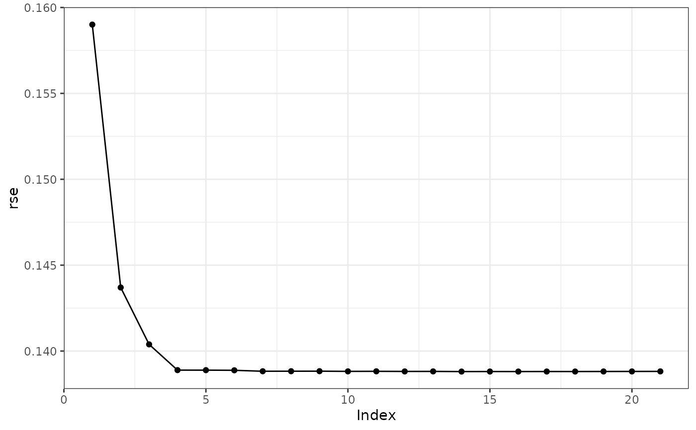 # preferable model is in index 5 by eye
preferable_cp <- cpr_run[["cps"]][[5]]
# }
#############################################################################
# Example 2: logistic regression
# simulate a binary response Pr(y = 1 | x) = p(x)
p <- function(x) { 0.65 * sin(x * 0.70) + 0.3 * cos(x * 4.2) }
set.seed(42)
x <- runif(2500, 0.00, 4.5)
sim_data <- data.frame(x = x, y = rbinom(2500, 1, p(x)))
# Define the initial control polygon
init_cp <- cp(formula = y ~ bsplines(x, df = 24, bknots = c(0, 4.5)),
data = sim_data,
method = glm,
method.args = list(family = binomial())
)
# run CPR
cpr_run <- cpr(init_cp)
#>
|
| | 0%
|
|=== | 5%
|
|======= | 10%
|
|========== | 14%
|
|============= | 19%
|
|================= | 24%
|
|==================== | 29%
|
|======================= | 33%
|
|=========================== | 38%
|
|============================== | 43%
|
|================================= | 48%
|
|===================================== | 52%
|
|======================================== | 57%
|
|=========================================== | 62%
|
|=============================================== | 67%
|
|================================================== | 71%
|
|===================================================== | 76%
|
|========================================================= | 81%
|
|============================================================ | 86%
|
|=============================================================== | 90%
|
|=================================================================== | 95%
|
|======================================================================| 100%
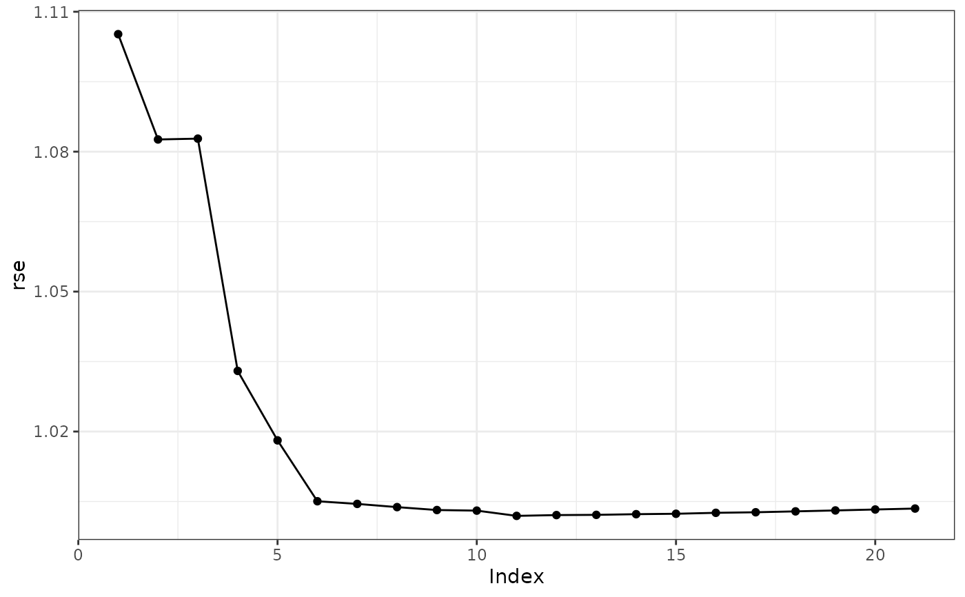
# preferable model is in index 6
s <- summary(cpr_run)
plot(s, color = TRUE, type = "rse")
# preferable model is in index 5 by eye
preferable_cp <- cpr_run[["cps"]][[5]]
# }
#############################################################################
# Example 2: logistic regression
# simulate a binary response Pr(y = 1 | x) = p(x)
p <- function(x) { 0.65 * sin(x * 0.70) + 0.3 * cos(x * 4.2) }
set.seed(42)
x <- runif(2500, 0.00, 4.5)
sim_data <- data.frame(x = x, y = rbinom(2500, 1, p(x)))
# Define the initial control polygon
init_cp <- cp(formula = y ~ bsplines(x, df = 24, bknots = c(0, 4.5)),
data = sim_data,
method = glm,
method.args = list(family = binomial())
)
# run CPR
cpr_run <- cpr(init_cp)
#>
|
| | 0%
|
|=== | 5%
|
|======= | 10%
|
|========== | 14%
|
|============= | 19%
|
|================= | 24%
|
|==================== | 29%
|
|======================= | 33%
|
|=========================== | 38%
|
|============================== | 43%
|
|================================= | 48%
|
|===================================== | 52%
|
|======================================== | 57%
|
|=========================================== | 62%
|
|=============================================== | 67%
|
|================================================== | 71%
|
|===================================================== | 76%
|
|========================================================= | 81%
|
|============================================================ | 86%
|
|=============================================================== | 90%
|
|=================================================================== | 95%
|
|======================================================================| 100%
# preferable model is in index 6
s <- summary(cpr_run)
plot(s, color = TRUE, type = "rse")
 plot(
cpr_run
, color = TRUE
, from = 5
, to = 7
, show_spline = TRUE
, show_cp = FALSE
)
#> Error in eval(expr): object 'cpr_run' not found
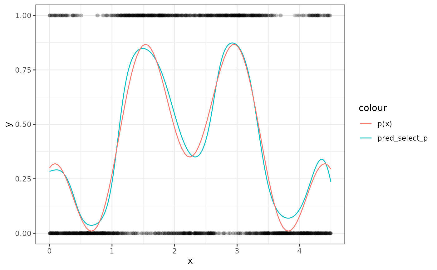
# plot the fitted spline and the true p(x)
sim_data$pred_select_p <- plogis(predict(cpr_run[[7]], newdata = sim_data))
ggplot2::ggplot(sim_data) +
ggplot2::theme_bw() +
ggplot2::aes(x = x) +
ggplot2::geom_point(mapping = ggplot2::aes(y = y), alpha = 0.1) +
ggplot2::geom_line(
mapping = ggplot2::aes(y = pred_select_p, color = "pred_select_p")
) +
ggplot2::stat_function(fun = p, mapping = ggplot2::aes(color = 'p(x)'))
plot(
cpr_run
, color = TRUE
, from = 5
, to = 7
, show_spline = TRUE
, show_cp = FALSE
)
#> Error in eval(expr): object 'cpr_run' not found
# plot the fitted spline and the true p(x)
sim_data$pred_select_p <- plogis(predict(cpr_run[[7]], newdata = sim_data))
ggplot2::ggplot(sim_data) +
ggplot2::theme_bw() +
ggplot2::aes(x = x) +
ggplot2::geom_point(mapping = ggplot2::aes(y = y), alpha = 0.1) +
ggplot2::geom_line(
mapping = ggplot2::aes(y = pred_select_p, color = "pred_select_p")
) +
ggplot2::stat_function(fun = p, mapping = ggplot2::aes(color = 'p(x)'))
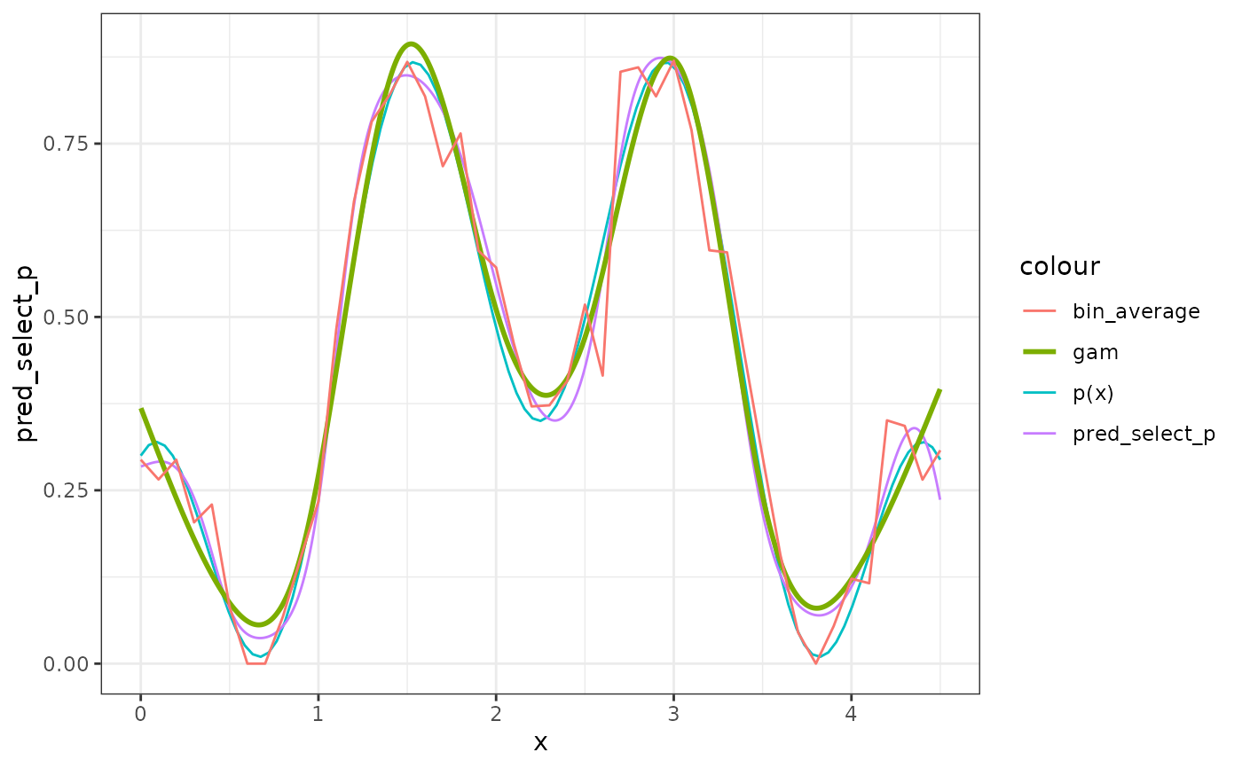
 # compare to gam and a binned average
sim_data$x2 <- round(sim_data$x, digits = 1)
bin_average <-
lapply(split(sim_data, sim_data$x2), function(x) {
data.frame(x = x$x2[1], y = mean(x$y))
})
bin_average <- do.call(rbind, bin_average)
ggplot2::ggplot(sim_data) +
ggplot2::theme_bw() +
ggplot2::aes(x = x) +
ggplot2::stat_function(fun = p, mapping = ggplot2::aes(color = 'p(x)')) +
ggplot2::geom_line(
mapping = ggplot2::aes(y = pred_select_p, color = "pred_select_p")
) +
ggplot2::stat_smooth(mapping = ggplot2::aes(y = y, color = "gam"),
method = "gam",
formula = y ~ s(x, bs = "cs"),
se = FALSE,
n = 1000) +
ggplot2::geom_line(data = bin_average
, mapping = ggplot2::aes(y = y, color = "bin_average"))
# compare to gam and a binned average
sim_data$x2 <- round(sim_data$x, digits = 1)
bin_average <-
lapply(split(sim_data, sim_data$x2), function(x) {
data.frame(x = x$x2[1], y = mean(x$y))
})
bin_average <- do.call(rbind, bin_average)
ggplot2::ggplot(sim_data) +
ggplot2::theme_bw() +
ggplot2::aes(x = x) +
ggplot2::stat_function(fun = p, mapping = ggplot2::aes(color = 'p(x)')) +
ggplot2::geom_line(
mapping = ggplot2::aes(y = pred_select_p, color = "pred_select_p")
) +
ggplot2::stat_smooth(mapping = ggplot2::aes(y = y, color = "gam"),
method = "gam",
formula = y ~ s(x, bs = "cs"),
se = FALSE,
n = 1000) +
ggplot2::geom_line(data = bin_average
, mapping = ggplot2::aes(y = y, color = "bin_average"))