Pediatric Blood Pressure Distributions
Source:vignettes/articles/bp-distributions_ARTICLE.Rmd
bp-distributions_ARTICLE.RmdIntroduction
Part of the work of Martin, DeWitt, Scott, et al. (2022) required transforming blood pressure measurement into percentiles based on published norms. This work was complicated by the fact that data for pediatric blood pressure percentiles is sparse and generally only applicable to children at least one year of age and requires height, a commonly unavailable data point in electronic health records for a variety of reasons.
A solution to building pediatric blood pressure percentiles was developed and is presented here for others to use. Inputs for the developed method are:
- Patient sex (male/female) required
- Systolic blood pressure (mmHg) required
- Diastolic blood pressure (mmHg) required
- Patient height (cm) if known.
Given the inputs, the following logic is used to determine which data sets will be used to inform the blood pressure percentiles. Under one year of age, the data from Gemelli et al. (1990) will be used; a height input is not required for this patient subset. For those at least one year of age with a known height, data from Expert Panel on Integrated Guidelines for Cardiovascular Health and Risk Reduction in Children and Adolescents (2011) (hereafter referred to as ‘NHLBI/CDC’ as the report incorporates recommendations and inputs from the National Heart, Lung, and Blood Institute [NHLBI] and the Centers for Disease Control and Prevention [CDC]). If height is unknown and age is at least three years, then data from Lo et al. (2013) is used. Lastly, for children between one and three years of age with unknown height, blood pressure percentiles are estimated by the NHLBI/CDC data using as a default the median height for each patient’s sex and age.

Estimating Pediatric Blood Pressure Distributions
There are two functions provided for working with blood pressure distributions. These methods use Gaussian distributions for both systolic and diastolic blood pressures with means and standard deviations either explicitly provided in an aforementioned source or derived by optimizing the parameters such that the sum of squared errors between the provided quantiles from an aforementioned source and the distribution quantiles is minimized. The provided functions, a distribution function and a quantile function, follow a similar naming convention to the distribution functions found in the stats library in R.
Arguments named p_sbp and p_dbp are
probabilities on the 0 to 1 scale. Arguments named
height_percentile and displayed percentiles in text or
plots use percentile points on the 0 to 100 scale.
args(p_bp)
## function (q_sbp, q_dbp, age, male, height = NA, height_percentile = NA,
##     default_height_percentile = 50, source = getOption("pedbp_bp_source",
##         "martin2022"), ...)
## NULL

# Quantile Function
args(q_bp)
## function (p_sbp, p_dbp, age, male, height = NA, height_percentile = NA,
##     default_height_percentile = 50, source = getOption("pedbp_bp_source",
##         "martin2022"), ...)
## NULL
Both methods expect an age in months and an indicator for sex.
height, in centimeters, is used preferentially over
height_percentile. The
default_height_percentile. is set to 50 by default to match
the flowchart above, but can be adjusted here to meet the end users
needs.
The reference look up tables for the Expert
Panel on Integrated Guidelines for Cardiovascular Health and Risk
Reduction in Children and Adolescents (2011) and Flynn et al. (2017) require height percentiles.
If height is entered, then the height percentile is
determined via an LMS method for age and sex using corresponding LMS
data from either the Centers for Disease control (CDC) or the World
Health Organization (WHO) based on age. Under 36 months use the WHO data
to estimate the height percentile and for 36 months and over use the CDC
data. The look up table will use the percentile nearest the calculated
value. Look up height percentiles values are: 5, 10, 25, 50, 75, 90, and
95.
If you want to restrict to CDC or WHO values regardless of age, we
recommend using p_height_for_age and
p_length_for_age to get height (stature) percentiles and
pass the result to the height_percentile argument.
Percentiles
What percentile for systolic and diastolic blood pressure is 100/60 for a 44 month old male with unknown height?
p_bp(q_sbp = 100, q_dbp = 60, age = 44, male = 1)
## $sbp_p
## [1] 0.7700861
##
## $dbp_p
## [1] 0.72739
Those percentiles would be modified if height was 103 cm:
p_bp(q_sbp = 100, q_dbp = 60, age = 44, male = 1, height = 103)
## $sbp_p
## [1] 0.7434636
##
## $dbp_p
## [1] 0.8678361
For the age and sex, the height of 103 is approximately the 79th percentile.
p_height_for_age(103, male = 1, age = 44)
## [1] 0.795653
x <- p_bp(q_sbp = 100, q_dbp = 60, age = 44, male = 1, height_percentile = 80, source = "nhlbi")
x
## $sbp_p
## [1] 0.7434636
##
## $dbp_p
## [1] 0.8678361
A plotting method to show where the observed blood pressures are on the distribution function is also provided.
bp_cdf(sbp = 90, dbp = 55, age = 44, male = 1, height = 103, source = "nhlbi")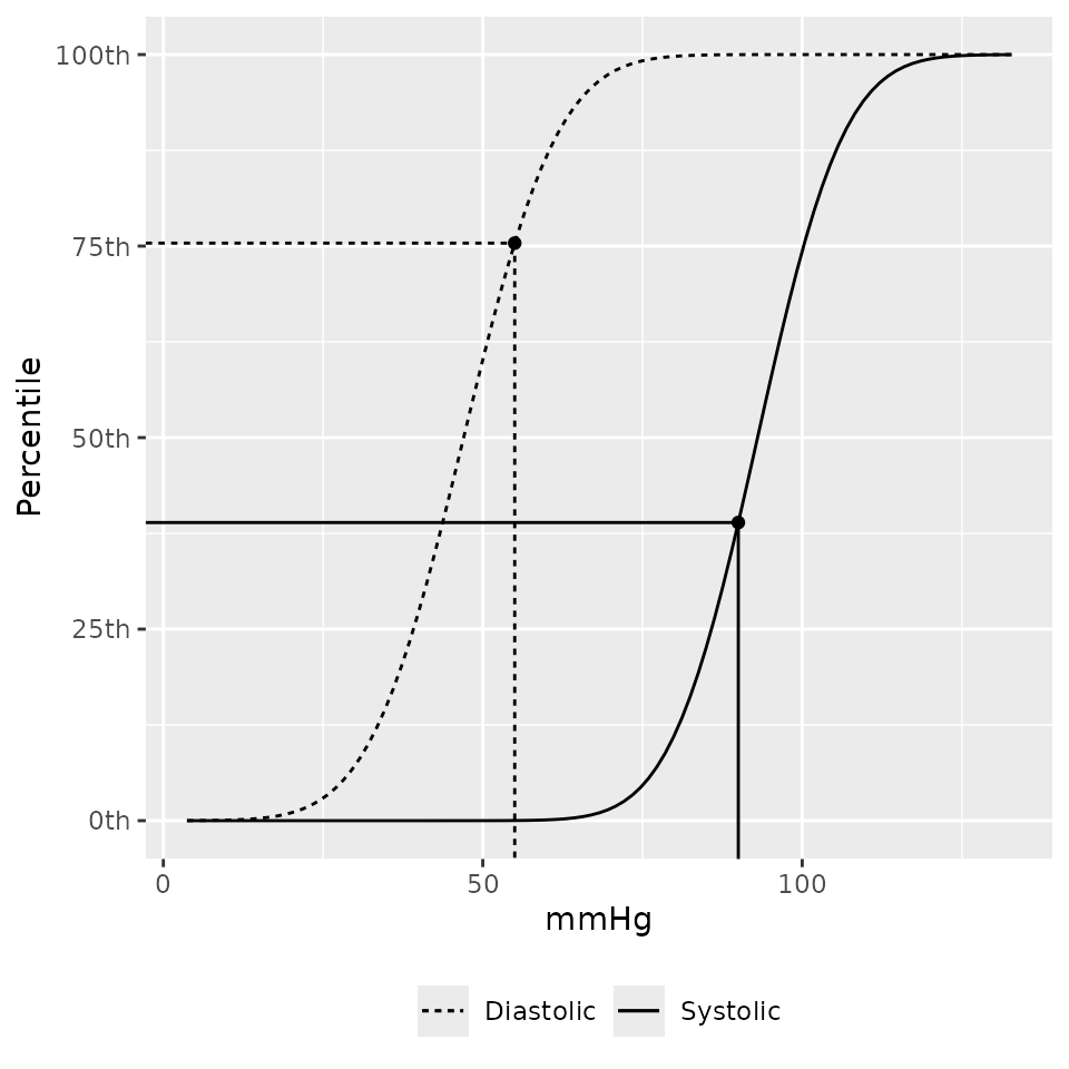
Vectors of blood pressures can be used as well. NA values will return NA.
bps <-
  p_bp(
         q_sbp  = c(100, NA, 90)
       , q_dbp  = c(60, 82, 48)
       , age    = 44
       , male   = 1
       , height_percentile = 80
      )
bps
## $sbp_p
## [1] 0.7434636        NA 0.3891471
##
## $dbp_p
## [1] 0.8678361 0.9986750 0.5341129
If you want to know which data source was used in computing each of
the percentile estimates you can look at the bp_params
attribute:
attr(bps, "bp_params")
##   source male age sbp_mean   sbp_sd dbp_mean   dbp_sd height_percentile
## 1  nhlbi    1  36 93.00921 10.68829 47.00316 11.64362                75
## 2  nhlbi    1  36 93.00921 10.68829 47.00316 11.64362                75
## 3  nhlbi    1  36 93.00921 10.68829 47.00316 11.64362                75
Quantiles
If you have a percentile value and want to know the associated systolic and diastolic blood pressures:
Working With More Than One Patient
The p_bp and q_bp methods are designed
accept vectors for each of the arguments. These methods expected each
argument to be length 1 or all the same length.
eg_data <- read.csv(system.file("example_data", "for_batch.csv", package = "pedbp"))
eg_data
##           pid age_months male height..cm. sbp..mmHg. dbp..mmHg.
## 1   patient_A         96    1          NA        102         58
## 2   patient_B        144    0         153        113         NA
## 3   patient_C          4    0          62         82         43
## 4 patient_D_1         41    1          NA         96         62
## 5 patient_D_2         41    1         101         96         62

bp_percentiles <-
  p_bp(
         q_sbp  = eg_data$sbp..mmHg.
       , q_dbp  = eg_data$dbp..mmHg.
       , age    = eg_data$age
       , male   = eg_data$male
       , height = eg_data$height
       )
bp_percentiles
## $sbp_p
## [1] 0.5533069 0.7680539 0.2622697 0.6195685 0.6101919
##
## $dbp_p
## [1] 0.4120704        NA 0.1356661 0.8028518 0.9011250

str(bp_percentiles)
## List of 2
##  $ sbp_p: num [1:5] 0.553 0.768 0.262 0.62 0.61
##  $ dbp_p: num [1:5] 0.412 NA 0.136 0.803 0.901
##  - attr(*, "bp_params")='data.frame':    5 obs. of  8 variables:
##   ..$ source           : chr [1:5] "lo2013" "nhlbi" "gemelli1990" "lo2013" ...
##   ..$ male             : int [1:5] 1 0 0 1 1
##   ..$ age              : num [1:5] 96 144 3 36 36
##   ..$ sbp_mean         : num [1:5] 100.7 105 89 93.2 93
##   ..$ sbp_sd           : num [1:5] 9.7 10.9 11 9.2 10.7
##   ..$ dbp_mean         : num [1:5] 59.8 62 54 55.1 47
##   ..$ dbp_sd           : num [1:5] 8.1 10.9 10 8.1 11.6
##   ..$ height_percentile: num [1:5] NA 50 NA NA 75
##  - attr(*, "class")= chr [1:2] "pedbp_bp" "pedbp_p_bp"
Going from percentiles back to quantiles:
q_bp(
       p_sbp  = bp_percentiles$sbp_p
     , p_dbp  = bp_percentiles$dbp_p
     , age    = eg_data$age
     , male   = eg_data$male
     , height = eg_data$height
     )
## $sbp
## [1] 102 113  82  96  96
##
## $dbp
## [1] 58 NA 43 62 62
Select Source Data
The default method for estimating blood pressure percentiles is based
on the method of Martin, DeWitt, Scott, et al.
(2022) and Martin, DeWitt, Albers, et al.
(2022) which uses three different references depending on age and
known/unknown stature. If you want to use a specific reference then you
can do so by using the source argument.
If you have a project with the want/need to use a specific source and you’d to use you can set it as an option:
options(pedbp_bp_source = "martin2022") # defaultThere are four sources:
- Gemelli et al. (1990) for kids under one year of age.
- Lo et al. (2013) for kids over three years of age and when height is unknown.
- Expert Panel on Integrated Guidelines for Cardiovascular Health and Risk Reduction in Children and Adolescents (2011) for kids 1 through 18 years of age with known stature.
- Flynn et al. (2017) for kids 1 through 18 years of age with known stature.
The data from Flynn et al. (2017) and Expert Panel on Integrated Guidelines for Cardiovascular Health and Risk Reduction in Children and Adolescents (2011) are similar but for one major difference. Flynn et al. (2017) excluded overweight and obese ( BMI above the 85th percentile) children.
For example, the estimated percentile for a blood pressure of 92/60 in a 39.2 month old female in the 95th height percentile are:
d <- data.frame(source = c("martin2022", "gemelli1990", "lo2013", "nhlbi", "flynn2017"),
                p_sbp = NA_real_,
                p_dbp = NA_real_)

for(i in 1:nrow(d)) {
  bp <- p_bp(q_sbp = 92, q_dbp = 60, age = 39.2, male = 0, height_percentile = 95, source = d$source[i])
  d[i, "p_sbp"] <- bp$sbp
  d[i, "p_dbp"] <- bp$dbp
}
d
##        source     p_sbp     p_dbp
## 1  martin2022 0.4612040 0.7950359
## 2 gemelli1990        NA        NA
## 3      lo2013 0.4703190 0.7017401
## 4       nhlbi 0.4612040 0.7950359
## 5   flynn2017 0.4623641 0.7698042
The estimated 85th quantile SBP/DBP for a 39.2 month old female, who is in the 95th height percentile are:
d <- data.frame(source = c("martin2022", "gemelli1990", "lo2013", "nhlbi", "flynn2017"),
                q_sbp = NA_real_,
                q_dbp = NA_real_)

for(i in 1:nrow(d)) {
  bp <- q_bp(p_sbp = 0.85, p_dbp = 0.85, age = 39.2, male = 0, height_percentile = 95, source = d$source[i])
  d[i, "q_sbp"] <- bp$sbp
  d[i, "q_dbp"] <- bp$dbp
}
d
##        source    q_sbp    q_dbp
## 1  martin2022 103.5868 62.31975
## 2 gemelli1990       NA       NA
## 3      lo2013 102.4425 64.30968
## 4       nhlbi 103.5868 62.31975
## 5   flynn2017 104.0844 62.83117
Comparing to Published Percentiles
The percentiles published in Expert Panel on Integrated Guidelines for Cardiovascular Health and Risk Reduction in Children and Adolescents (2011) and Flynn et al. (2017) where used to estimate a Gaussian mean and standard deviation. This was in part to be consistent with the values from Gemelli et al. (1990) and Lo et al. (2013). As a result, the calculated percentiles and quantiles from the pedbp package for Expert Panel on Integrated Guidelines for Cardiovascular Health and Risk Reduction in Children and Adolescents (2011) and Flynn et al. (2017) will be slightly different from the published values.
Flynn et al.
fq <-
  q_bp(
     p_sbp = flynn2017$bp_percentile/100,
     p_dbp = flynn2017$bp_percentile/100,
     male  = flynn2017$male,
     age   = flynn2017$age,
     height_percentile = flynn2017$height_percentile,
     source = "flynn2017")

fp <-
  p_bp(
     q_sbp = flynn2017$sbp,
     q_dbp = flynn2017$dbp,
     male  = flynn2017$male,
     age   = flynn2017$age,
     height_percentile = flynn2017$height_percentile,
     source = "flynn2017")

f_bp <-
  cbind(flynn2017,
        pedbp_sbp = fq$sbp,
        pedbp_dbp = fq$dbp,
        pedbp_sbp_p = fp$sbp_p * 100,
        pedbp_dbp_p = fp$dbp_p * 100
  )
All the quantile estimates are within 2 mmHg:
summary(f_bp$pedbp_sbp - f_bp$sbp)
##      Min.   1st Qu.    Median      Mean   3rd Qu.      Max.
## -1.895796 -0.203214 -0.003978 -0.031863  0.085968  0.749248
summary(f_bp$pedbp_dbp - f_bp$dbp)
##      Min.   1st Qu.    Median      Mean   3rd Qu.      Max.
## -1.579830 -0.203214  0.004458  0.006043  0.158121  1.126966
All the percentiles estimates are within are within 2 percentile points:
summary(f_bp$pedbp_sbp_p - f_bp$bp_percentile)
## Min. 1st Qu. Median Mean 3rd Qu. Max.
## -0.99754 -0.14851 0.01554 0.02097 0.20186 1.69706
summary(f_bp$pedbp_dbp_p - f_bp$bp_percentile)
## Min. 1st Qu. Median Mean 3rd Qu. Max.
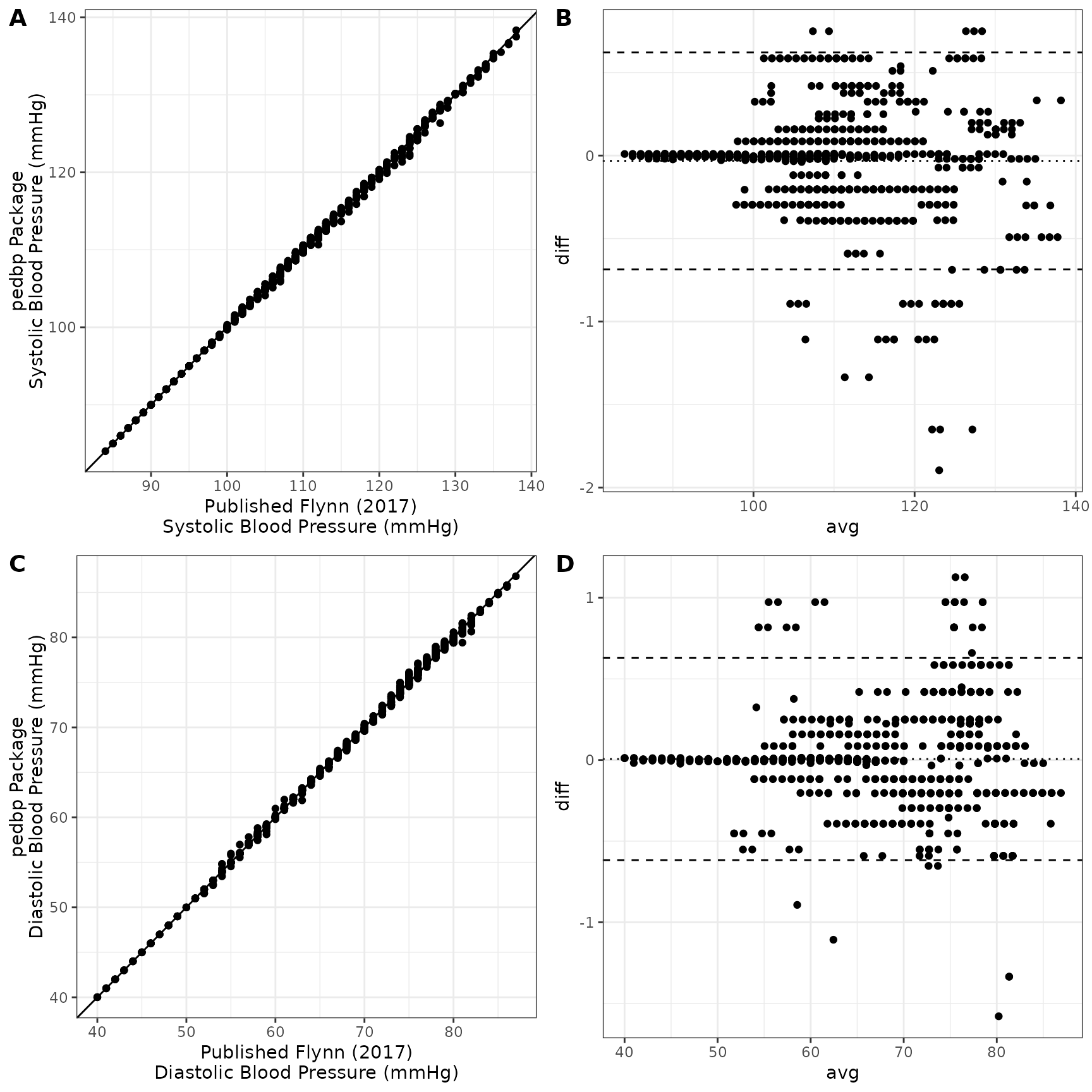
## -1.2203874 -0.2836688 -0.0191912 0.0001719 0.2212839 1.6970586A helpful set of graphics are shown below. Panels A and C show the estimated blood pressure quantiles provide by the pedbp package (y-axis) against the published quantiles from Flynn et al. (2017) for systolic and diastolic blood pressures respectively. Panels B and D are Bland-Altman plots showing the difference vs average between the two estimates.
NHLBI/CDC
nq <-
  q_bp(
     p_sbp = nhlbi_bp_norms$bp_percentile/100,
     p_dbp = nhlbi_bp_norms$bp_percentile/100,
     male  = nhlbi_bp_norms$male,
     age   = nhlbi_bp_norms$age,
     height_percentile = nhlbi_bp_norms$height_percentile,
     source = "nhlbi")

np <-
  p_bp(
     q_sbp = nhlbi_bp_norms$sbp,
     q_dbp = nhlbi_bp_norms$dbp,
     male  = nhlbi_bp_norms$male,
     age   = nhlbi_bp_norms$age,
     height_percentile = nhlbi_bp_norms$height_percentile,
     source = "nhlbi")

nhlbi_bp <-
  cbind(nhlbi_bp_norms,
        pedbp_sbp = nq$sbp,
        pedbp_dbp = nq$dbp,
        pedbp_sbp_p = np$sbp_p * 100,
        pedbp_dbp_p = np$dbp_p * 100
  )
All the quantile estimates are within 2 mmHg:
summary(nhlbi_bp$pedbp_sbp - nhlbi_bp$sbp)
##      Min.   1st Qu.    Median      Mean   3rd Qu.      Max.
## -1.199728 -0.173883 -0.003333 -0.014070  0.091753  0.817752
summary(nhlbi_bp$pedbp_dbp - nhlbi_bp$dbp)
##       Min.    1st Qu.     Median       Mean    3rd Qu.       Max.
## -1.0537249 -0.0357386  0.0009374 -0.0011066  0.0902619  1.0295371
All the percentiles are within 2 percentile points:
summary(nhlbi_bp$pedbp_sbp_p - nhlbi_bp$bp_percentile)
## Min. 1st Qu. Median Mean 3rd Qu. Max.
## -0.595528 -0.103685 0.005356 0.004987 0.058757 0.520902
summary(nhlbi_bp$pedbp_dbp_p - nhlbi_bp$bp_percentile)
## Min. 1st Qu. Median Mean 3rd Qu. Max.
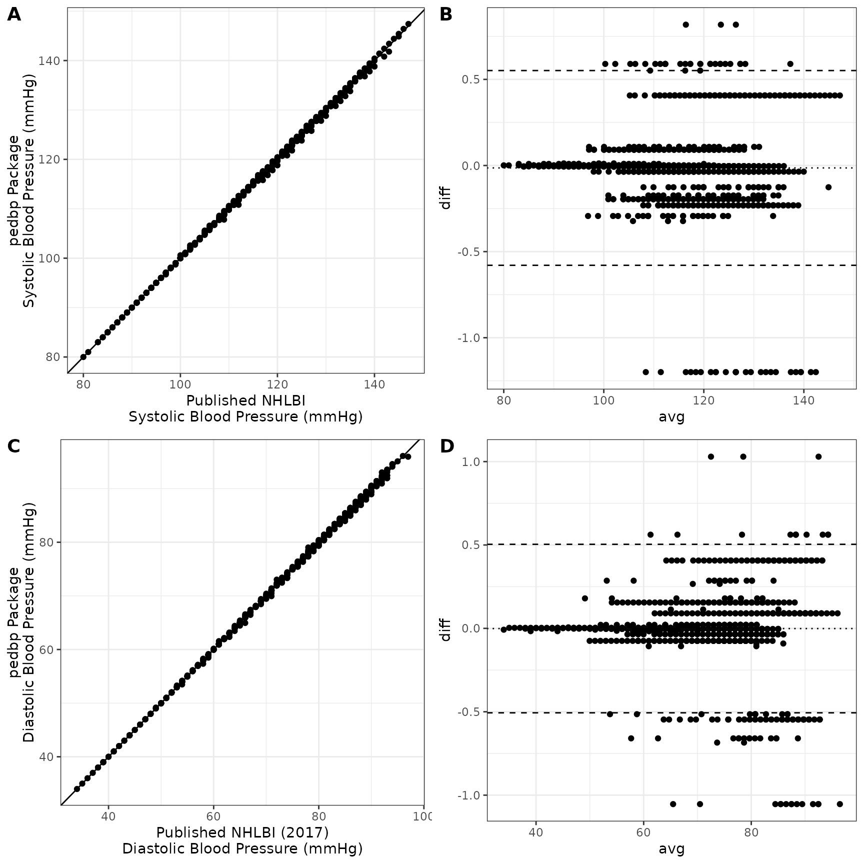
## -0.457032 -0.033946 -0.003424 0.001301 0.033660 0.602561A helpful set of graphics are shown below. Panels A and C show the estimated blood pressure quantiles provide by the pedbp package (y-axis) against the published quantiles from Expert Panel on Integrated Guidelines for Cardiovascular Health and Risk Reduction in Children and Adolescents (2011) for systolic and diastolic blood pressures respectively. Panels B and D are Bland-Altman plots showing the difference vs average between the two estimates.
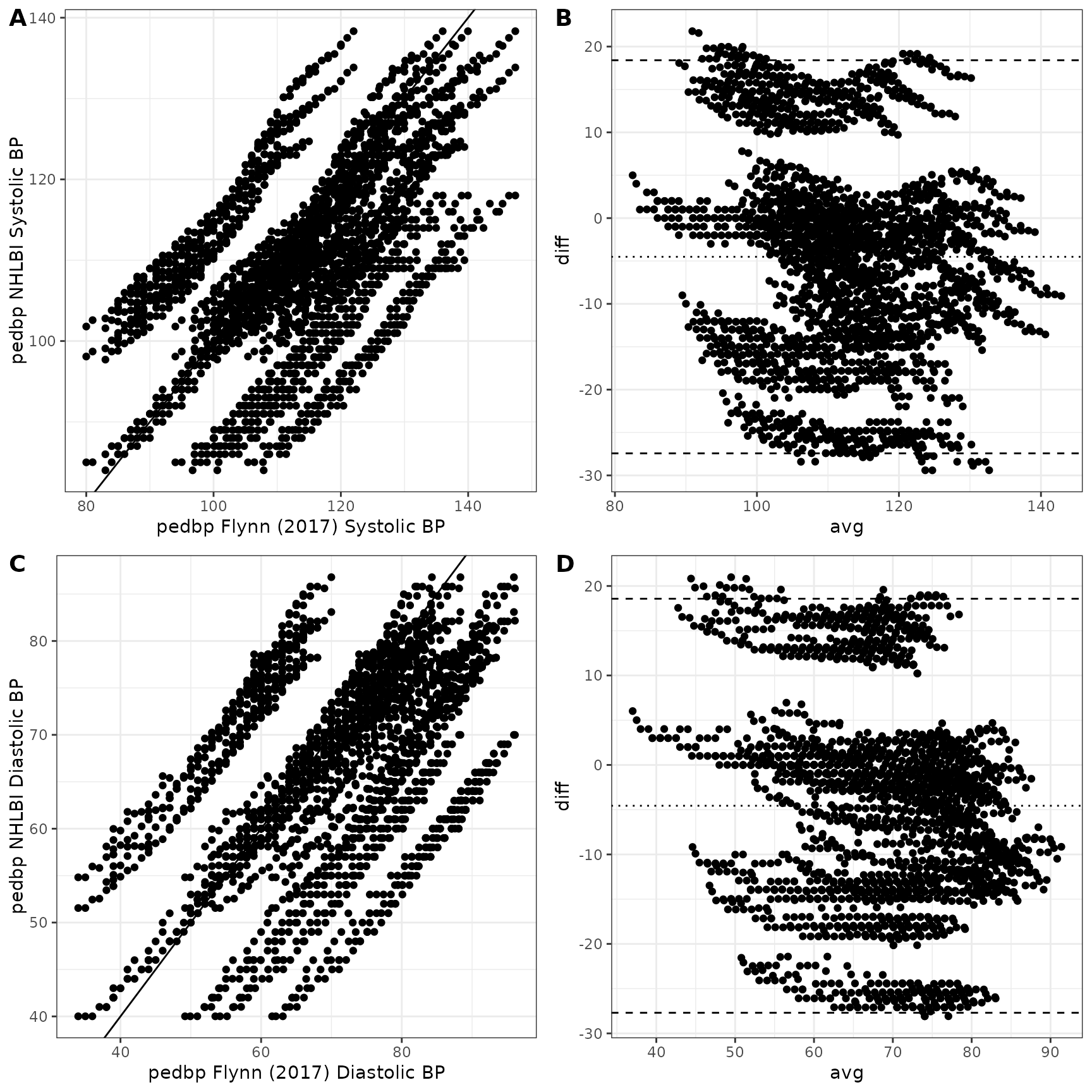
NHLBI vs Flynn 2017
The NHLBI data included overweight and obese children whereas Flynn excluded them. As a result, the estimates for blood pressures can differ significantly between the two sources.
The graphic below shows the estimated systolic and diastolic blood pressures provided by the pedbp package. As expected, the values estimated based on Flynn are lower, on average, than those estimated by data from the NHLBI.
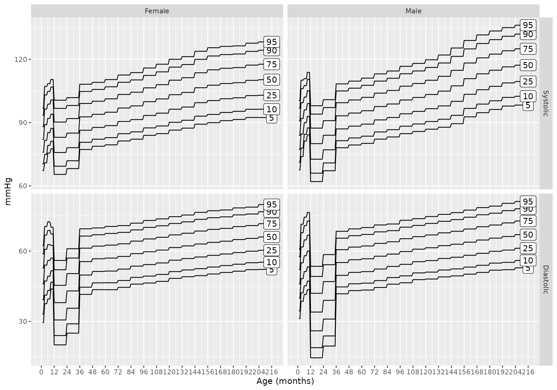
Blood Pressure Charts
To you can get blood pressure charts for any combination of inputs
using bp_chart. For example, the blood pressure percentiles
when using source = 'martin2022' and height is unknown
are:
And if height is known (say it is the 25th percentile)
bp_chart(p = c(0.05, 0.1, 0.25, 0.5, 0.75, 0.90, 0.95),
         height_percentile = 25,
         source = "martin2022")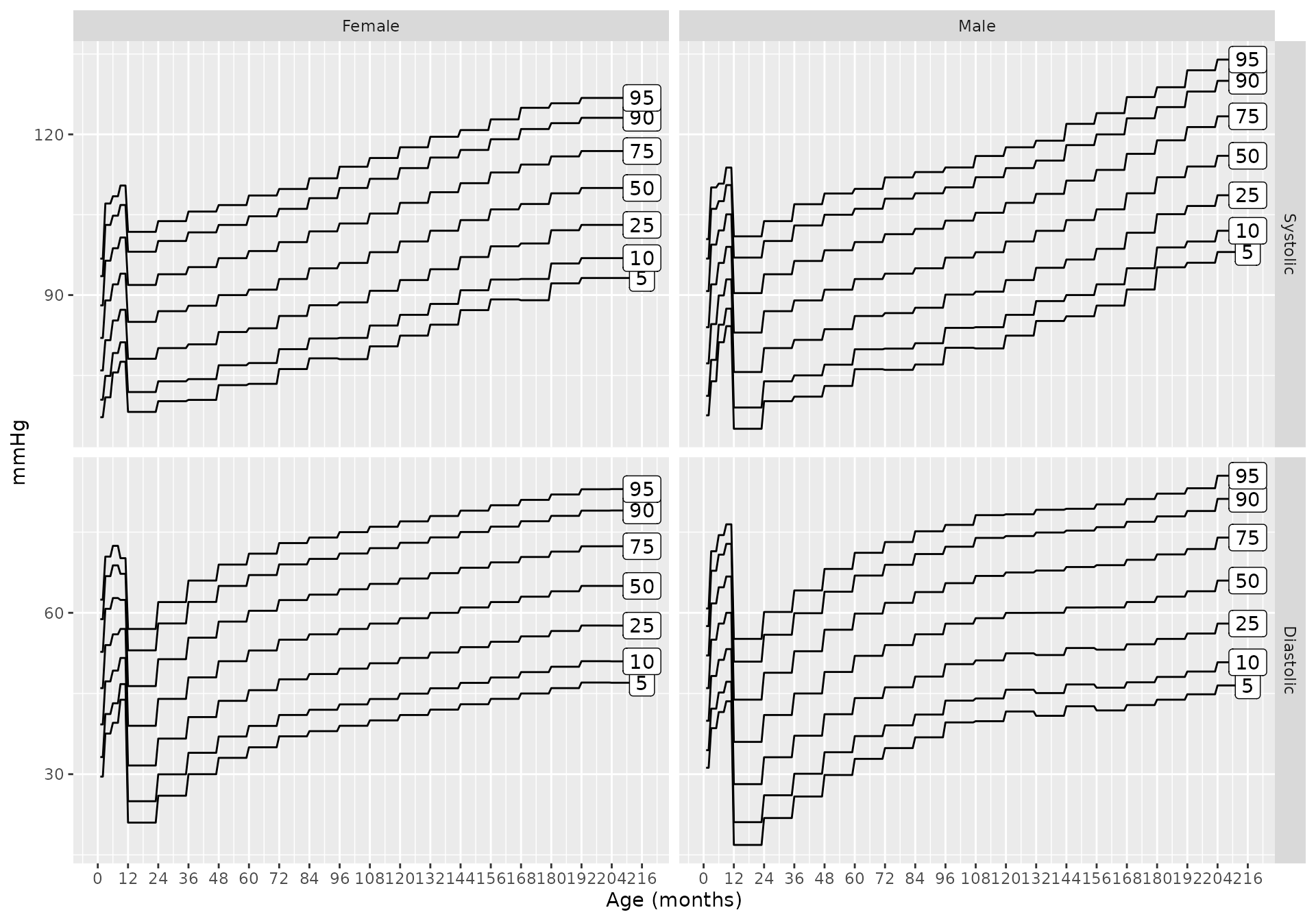
Additionally, charts for each of the specific data sources can be generated
bp_chart(source = "gemelli1990")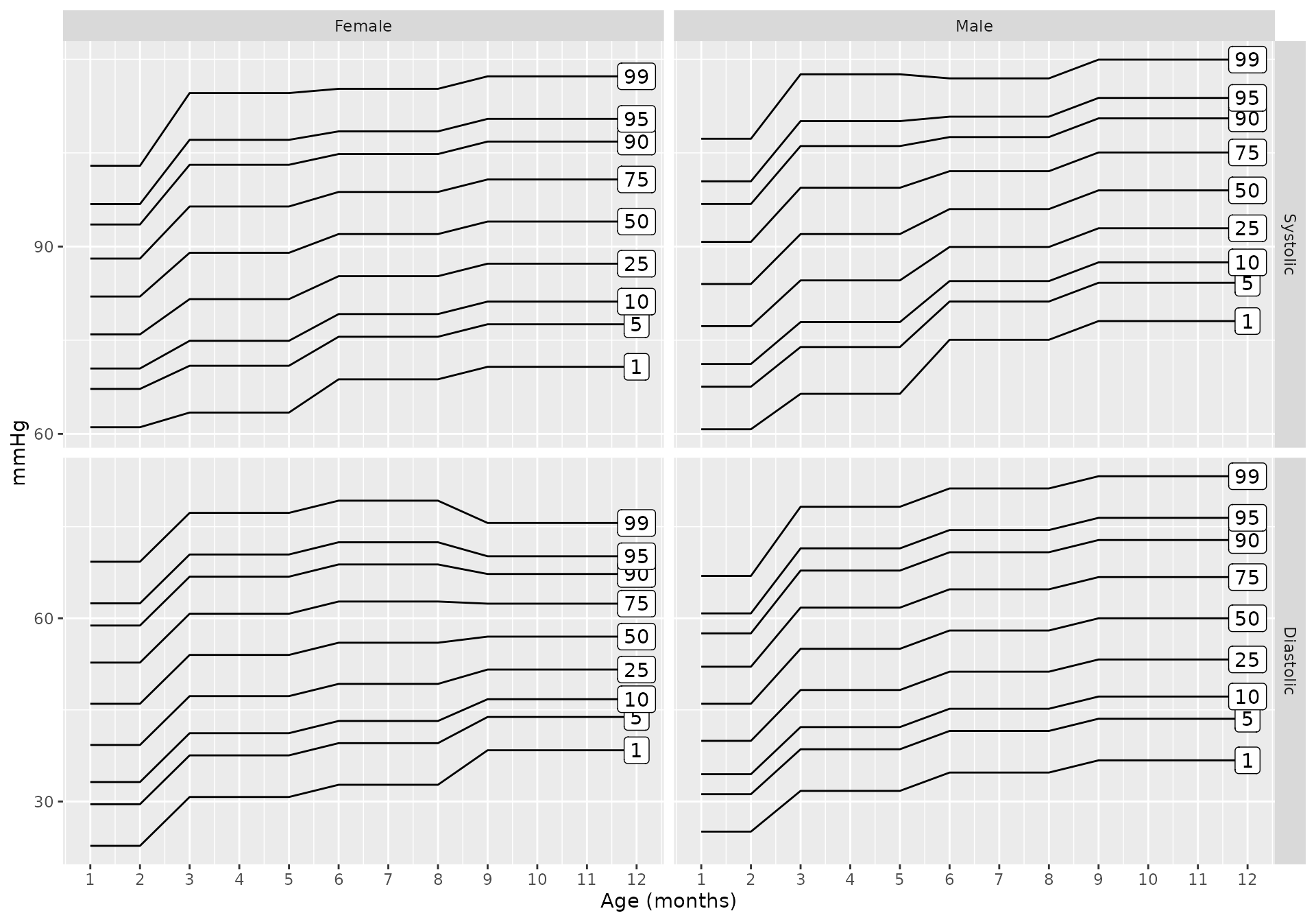
bp_chart(source = "lo2013")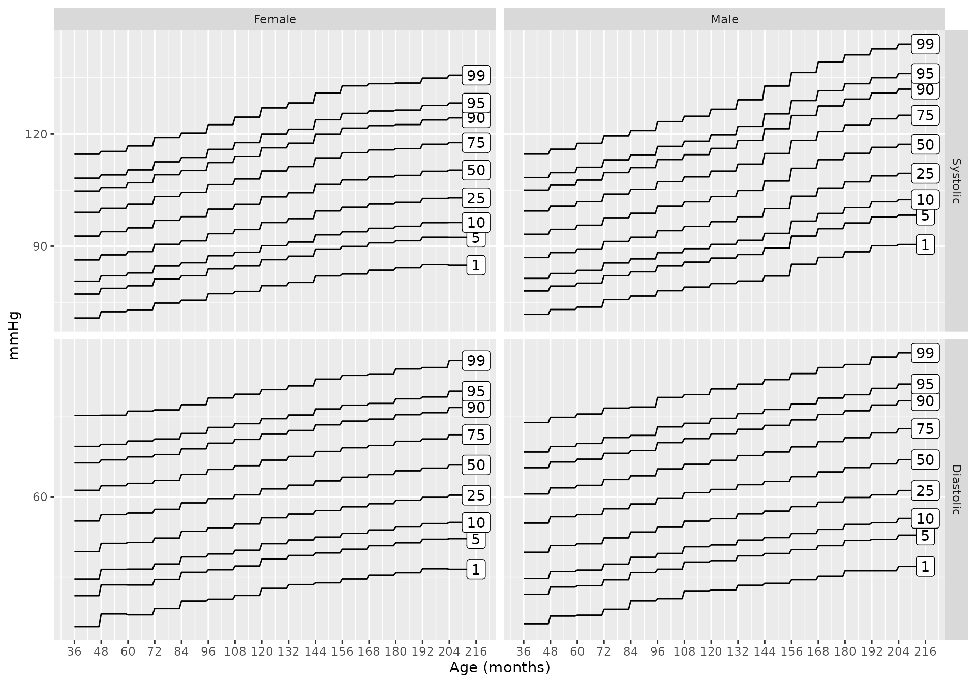
bp_chart(source = "nhlbi")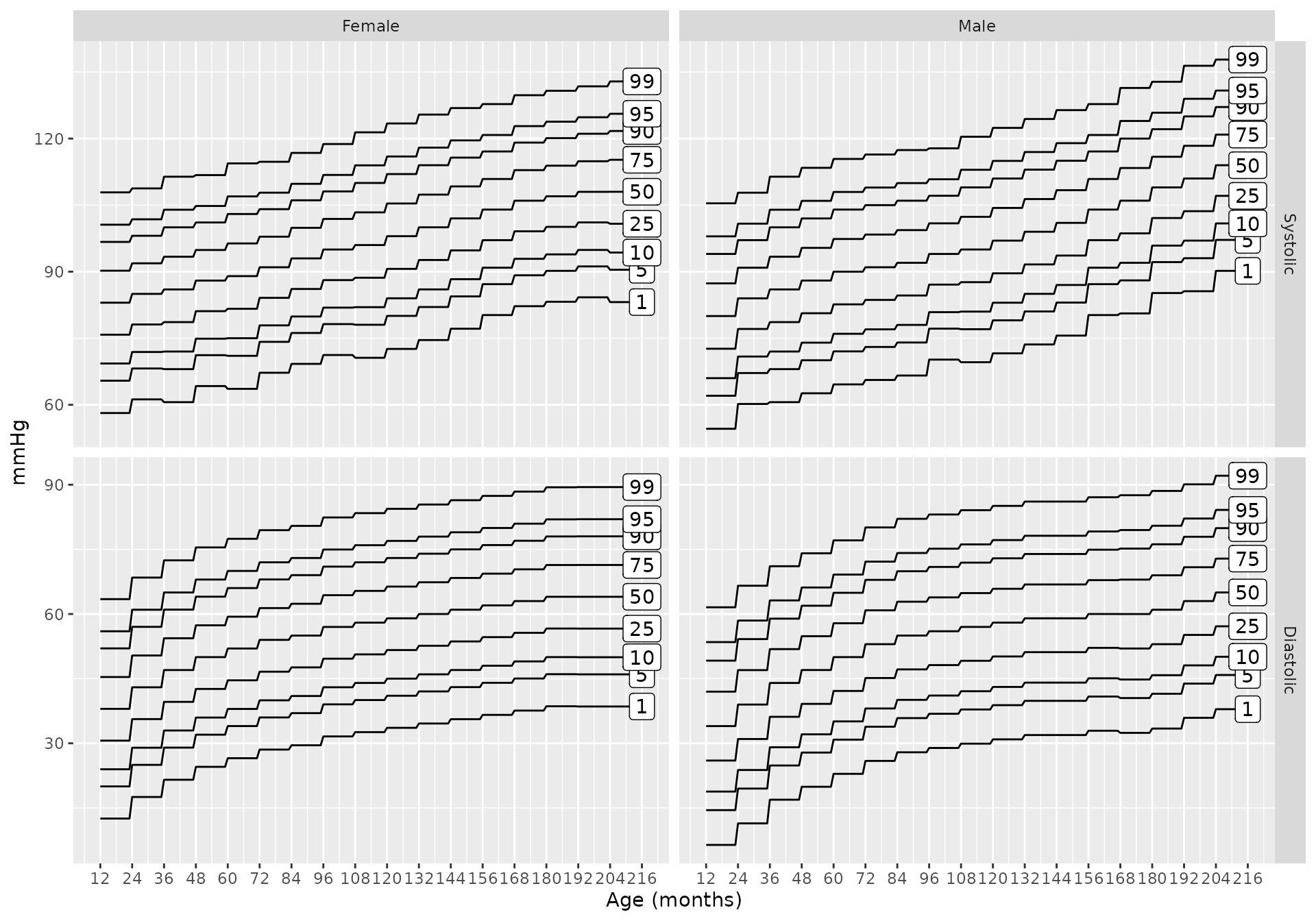
bp_chart(source = "flynn2017")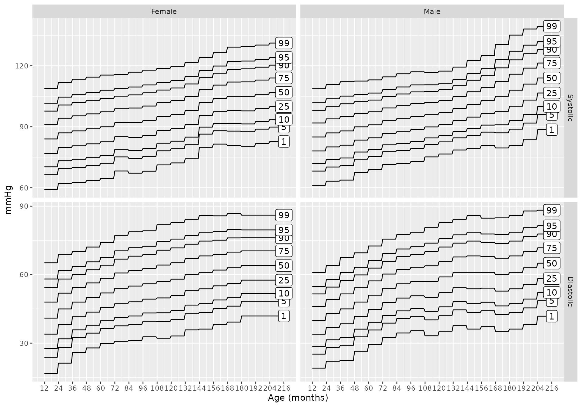
Shiny Application
An interactive Shiny application is also available. After installing the pedbp package and the suggested packages, you can run the app locally via
shiny::runApp(system.file("shinyapps", "pedbp", package = "pedbp"))The shiny application allows for interactive exploration of blood pressure percentiles for an individual patient and allows for batch processing a set of patients as well.